I have now reached the data visualization course in DataQuest’s Data Analyst in R track. I am really excited to have reached this point because I’ve always wanted to try visualizing data. One thing I like about data visualization is that it easier to identify patterns in data and plan analyses.
Throughout this course, I’ll be using a very popular tidyverse package called ggplot2. I follow the #rstats and #TidyTuesday hashtags on Twitter and ggplot2 is a package that I’ve seen discussed A LOT when it comes to data visualization in R. DataQuest attributes its popularity to its consistent syntax and the efficiency with which you can use to create quality data visualizations.
In this post, I am using yet another data set I found on Tidy Tuesday’s github repo. This data set explores bridges in the state of Maryland. Before I started with the lesson I made sure to load the tidyverse package, which includes gglplot2 and import the data, saving the data into a data frame called bmore_bridges. As shown in the screenshot below, I then filtered the data frame to only contain bridges owned by the State Highway Agency.
bmore_bridges_filter <- bmore_bridges %>% filter(owner == "State Highway Agency")
bmore_bridges_filter
# A tibble: 913 x 13
     lat  long county carries yr_built bridge_condition
   <dbl> <dbl> <chr>  <chr>      <dbl> <chr>
 1  39.2 -76.7 Anne … IS 695      1958 Fair
 2  39.2 -76.7 Anne … IS 695      1951 Fair
 3  39.2 -76.6 Anne … IS 695…     1957 Fair
 4  39.2 -76.6 Anne … IS 695…     1957 Fair
 5  39.2 -76.6 Anne … MD 2        1937 Good
 6  39.1 -76.6 Anne … MD 2        1936 Fair
 7  39.0 -76.5 Anne … MD 2 R…     1953 Good
 8  39.0 -76.5 Anne … US 50 …     1953 Fair
 9  39.0 -76.6 Anne … MD 2        1983 Fair
10  39.2 -76.7 Anne … MD 168      1949 Fair
# … with 903 more rows, and 7 more variables:
#   avg_daily_traffic <dbl>, total_improve_cost_thousands <dbl>,
#   inspection_mo <chr>, inspection_yr <dbl>, owner <chr>,
#   responsibility <chr>, vehicles <chr>
The first lesson in this course is about creating line graphs. The first topic that I went over was using plots to visualize data patterns. Plots are visual representations that use graphics like dots, lines, and bars to help you look for patterns in data. There are many kinds of plots I can use to visualize data. In this lesson, I used a line chart which is a type of plot that is especially useful for visualizing changes over time.
ggPlot2
So what’s the history behind ggplot2? Hadley Wickham, the chief data scientist at RStudio developed ggplot2 based on “Grammar of Graphics”. Grammar of Graphics, by Leland Wilkinson, refers to a system for data visualization.
Now that we know a bit of the history, I want go over step-by-step how I created my line chart.
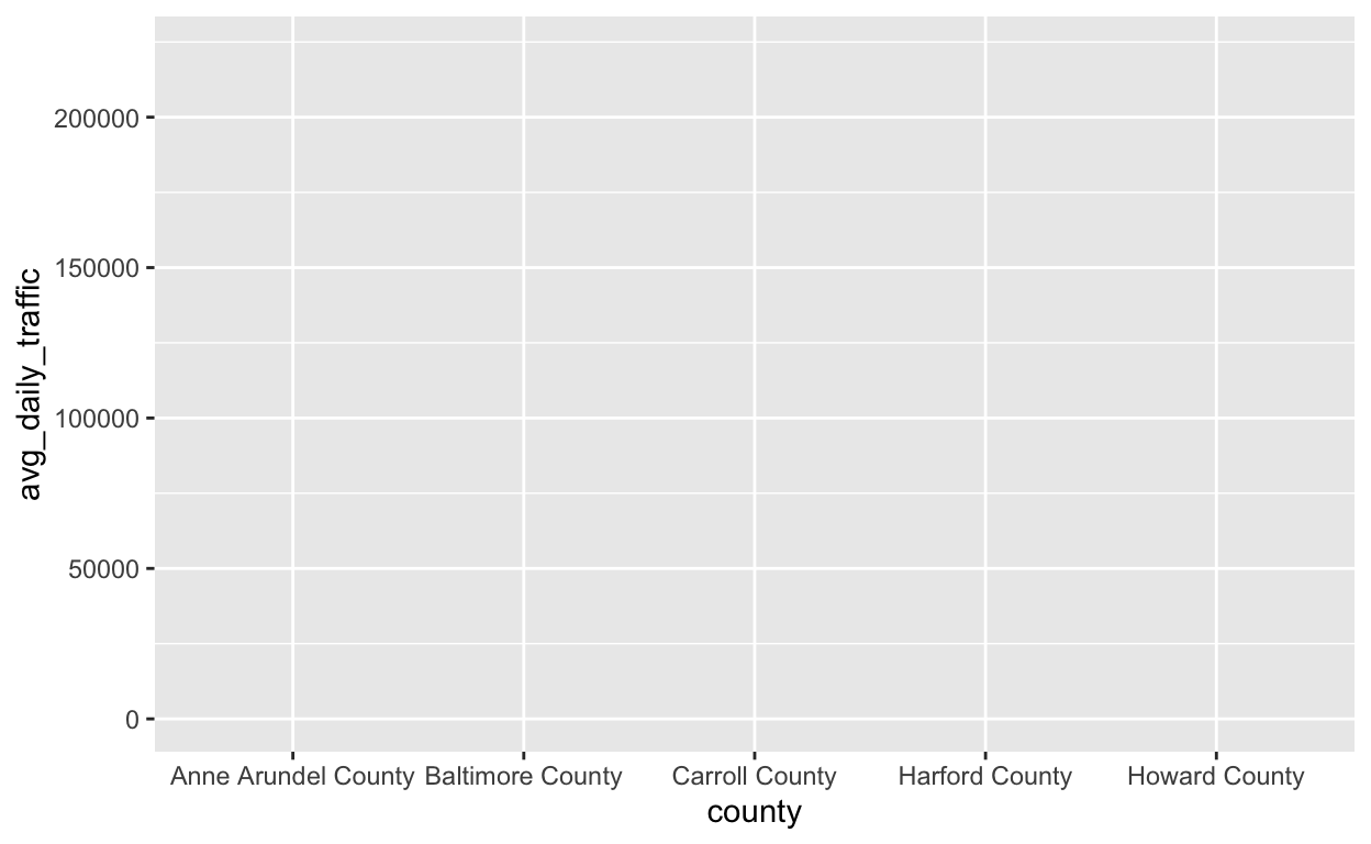
First, I begin to make a plot using the ggplot() function and specify the data frame I’ll be visualizing from. This step is the foundation in creating a coordinate system that I can add layers to. When I type the code below, I’ll get a graphic of an empty plot.
ggplot(data = bmore_bridges_filter)

Note: DataQuest notes that while I do not have to assign the data frame to the variable data, they recommend doing so as I learn ggplot(). It helps keep track of the different functions used to build data visualizations.
Aesthetics
The second step is to define the variables I want to map on my graph. To do this, I use the aes() function, which stands for aesthetics. Because I’m graphing dimensional data, my graph will have two axes: an x-axis and a y-axis. As shown here, I assigned the county variable to x and the avg_daily_traffic to y.
ggplot(data = bmore_bridges_filter) +
  aes(x = county, y = avg_daily_traffic)
But how do I know which axis to use for which variable? Let me explain.
- The variable that changes depending on another variable is called the dependent variable. This variable is assigned to the vertical axis, or y-axis. In the example above, avg_daily_traffic is the dependent variable because it changes depending on the county.
- The variable that changes independent of another variable is called the independent variable. This variable is assigned to the horizontal axis, or x-axis. In this case, county is the independent variable because its changes do not depend on another variable.
Also, from the photo shown there is a plus sign added at the end of the ggplot() function. To add new layers to the graph, a plus sign is needed followed by another layer.
Adding Geometric Objects to Visualize Data Points
The third step is to add geometric symbols to the graph to represent data points. As shown below, I added the geom_line() layer to my graph to add a line representing the relationship between the county and avg_daily_traffic variables.
ggplot(data = bmore_bridges_filter) +
  aes(x = county, y = avg_daily_traffic) +
  geom_line()
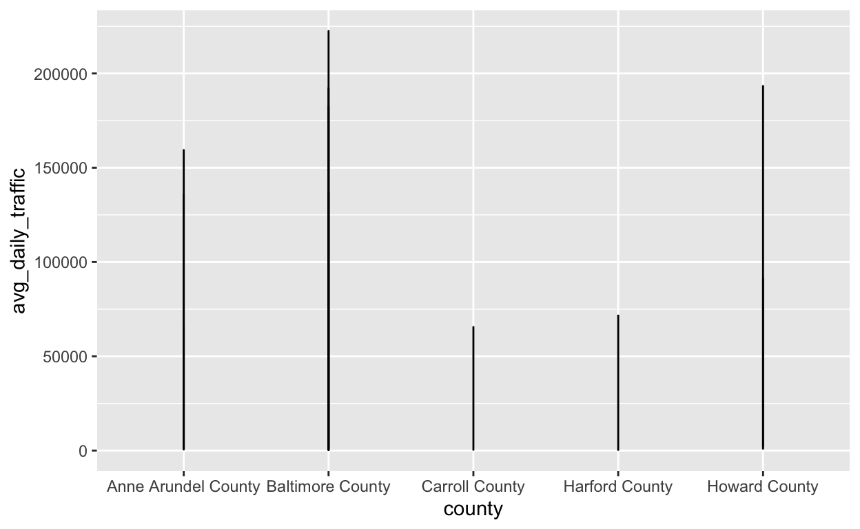
There are many types of geometric objects I could add to a graph depending on what type of data I’m working with the relationship between variables I’m looking to explore. But for this post, I focused on adding a line to visualize the data.
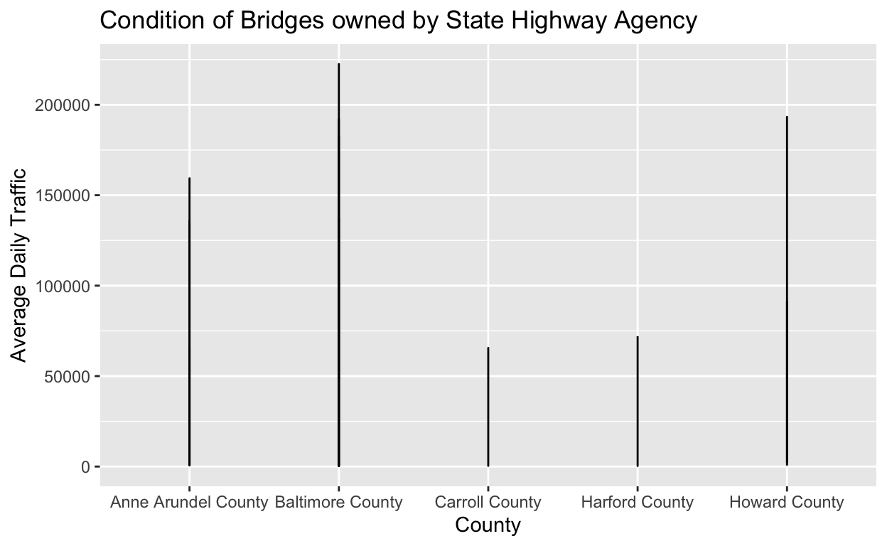
Adding Graph Titles and Axis Labels
I want to make my graph easier to understand. This is where adding graph titles and changing axis labels come in. The labs() layer, which is short for labels, is the next layer I added to my graph. I specified the title of my graph using title = , the x-axis , and the y-axis all inside the labs() argument. The titles and labels of a graph should be descriptive and clearly communicate the type of data used in the graph.
ggplot(data = bmore_bridges_filter) +
  aes(x = county, y = avg_daily_traffic) +
  geom_line() +
  labs(title = "Condition of Bridges owned by State Highway Agency", x= "County", y ="Average Daily Traffic")
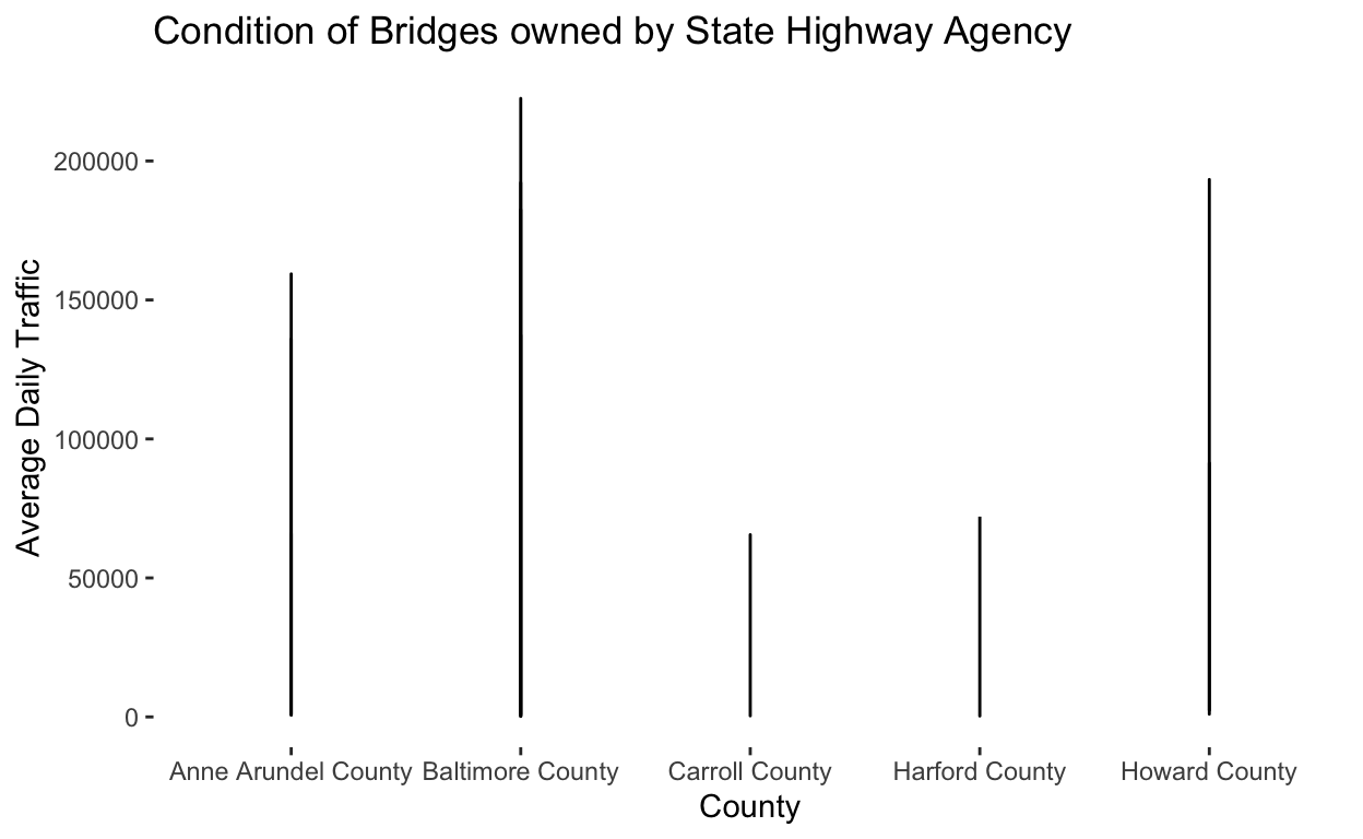
Refining Graph Aesthetics
So, I want to change the background color of my graph to white. To do this, I add another layer to my graph using the theme() layer. The theme() layer is used to modify non-data ggplot2 graph components. The argument panel.background = element_rect, specifies the color of the background rectangle(“rect” stands for rectangle). I then use fill = to specify that I want a white background.
The Final Result
When I run the following code, I get the following plot below. This is a basic, bare bones line chart but its clear and informative(I think). From this plot, I can see that Baltimore County has the highest average daily traffic and Carroll County has the lowest average daily traffic.
ggplot(data = bmore_bridges_filter) +
  aes(x = county, y = avg_daily_traffic) +
  geom_line() +
  labs(title = "Condition of Bridges owned by State Highway Agency", x= "County", y ="Average Daily Traffic") +
  theme(panel.background = element_rect(fill = 'white'))
The End
I can’t tell you enough how I excited I was about this part of the course. When I would look at #TidyTuesday posts, I would marvel at the creations people came up with. Though if I’m being honest, I was intimidated by the code. The more I code in R, the more I read others’ R code, the less intimidating the code is. I knew that I wanted to start creating cool data visualizations like the ones I admired. With these R lessons, I’m on my way to doing just that.
Well, that’s all I got for this lesson! Until next time…